Joe Ardent 38dac45d85 fix off-by-10x in scale analogy for accurate shasta

2023-01-21 15:56:38 -08:00

48 KiB

Raw Blame History

+++ title = "A Thoroughly Digital Artifact" slug = "a-thoroughly-digital-artifact" date = "2023-01-19" updated = "2023-01-21" [taxonomies] tags = ["3dprinting", "CAD", "GIS", "CNC", "art", "sundry", "proclamation", "research"] +++

A birthday wish

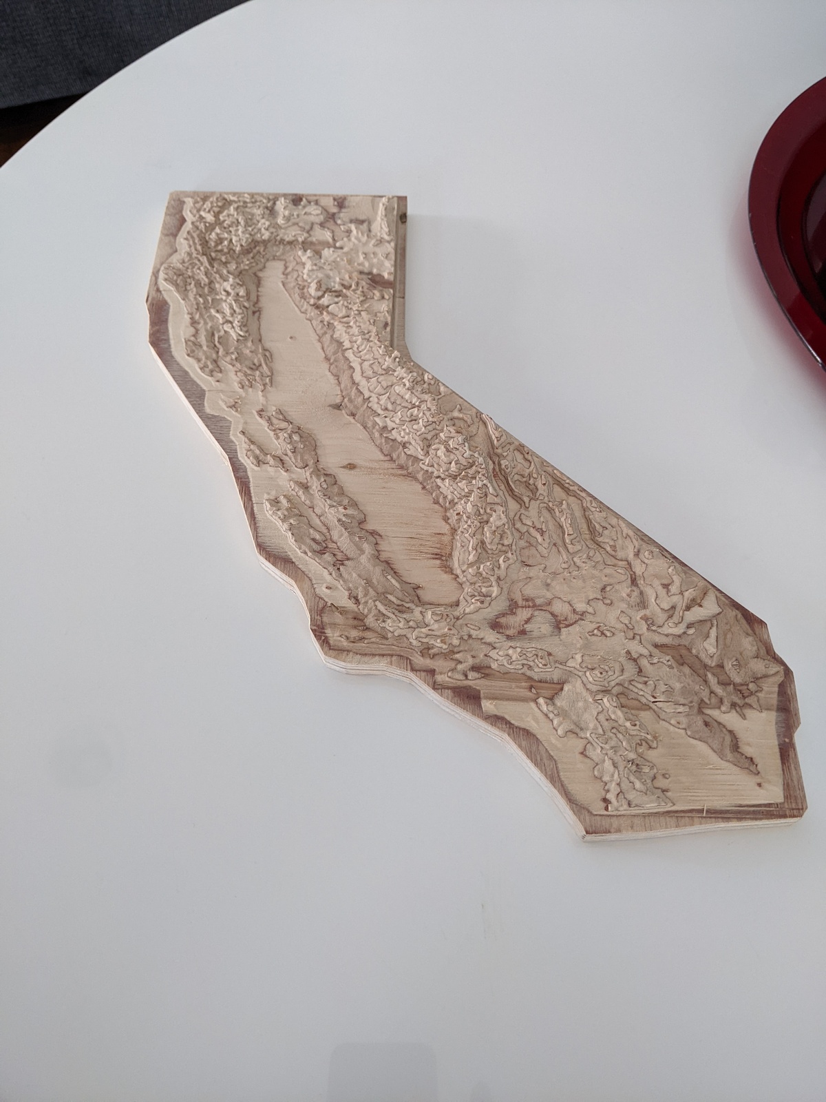
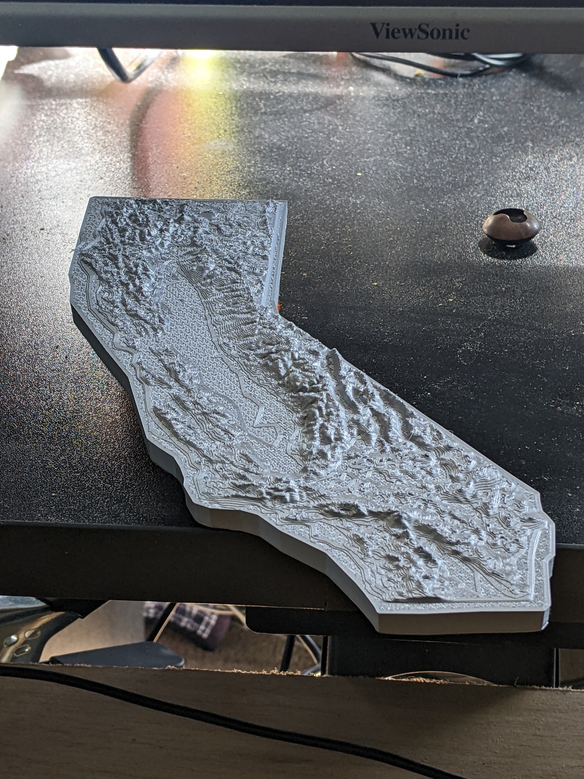
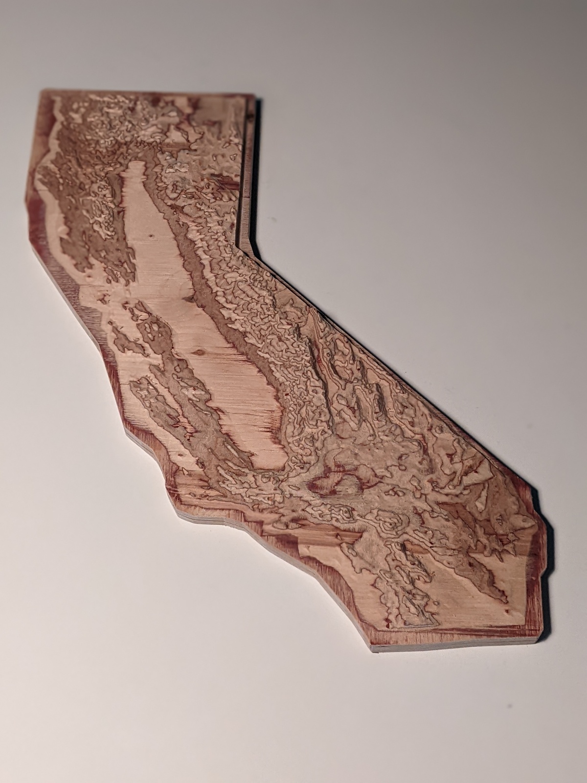
Last summer, I wanted to get my wife something nice for her birthday. For many years, she had expressed an occasional and casual desire for a topographic carving of the state of California, where we live, and I thought it might be something I could figure out how to get her. In the end, after many dozens of hours of work, five weeks, and several hundred dollars paid to a professional CNC machine shop, I had the artifact shown in the picture above. This is the story of its creation, starting from knowing almost nothing about GIS, cartography, or CNC machining.

First steps

Before you ask, I did not do a ton of research before embarking on this. As I write this, about six months later, it only now occurred to me to do a basic search for an actual physical thing I could buy, and luckily it seems that CNC-carved wooden relief maps of the whole state are not trivially easy to come by, so, phew!

No, my first step was to see if there were any shops in the area that could carve something out of nice plywood, about a week before the intended recipient's birthday. I found one that was less than ten minutes away, and filled out their web contact form. They had a field for material, and I said, "some nice plywood between 0.75 and 1.0 inches thick or similar" (I didn't know exactly what was available and wanted to give broad acceptable parameters), and under "project description", I wrote,

A relief map of California, carved from wood. Height exaggerated enough to visibly discern the Santa Monica mountains. I can provide an STL file if needed.

For some [incorrect] reason that I only later examined¹, I just sort of assumed that the shop would have a library of shapes available for instantiating into whatever material medium you might need. But just in case, I included that hedge about being able to provide an STL file. Needless to say, that was a bluff.

^{_{me, every. single. time.}}

Also needless to say, my bluff was immediately called, and I had the following exchange with the shop:

CNC Shop: STL can work but I can’t manipulate it, which could save some money. If possible can it be exported to an .igs or .iges or .stp format?

Me: Yeah, STP should be no problem. Can you give a rough estimate of the cost for 1x2-foot relief carving?

Shop: Without seeing the drawings, I can’t give even a close price but in the past they range from a few hundred dollars to several thousand dollars.

Me: That's totally fair! I'll get you some files in a few days.

"STP should be no problem ... I'll get you some files in a few days," was an even harder lean into the bluff; my next communication with the shop was nearly four weeks later. But that's getting ahead of things.

Meshes and solid bodies

First off, let's talk about file formats and how to represent shapes with a computer.² I first said I could provide an STL file. STL is a pretty bare-bones format that describes the outside surface of a shape as a mesh of many, many triangles, each of which is described by three 3D points, where each point (but not necessarily each edge) of the triangle lies on the surface of the shape of the thing you're modeling. This format is popular with 3D printers, which is how I became familiar with it.

STL is simple to implement and easy for a computer to read, but if you have a model in that format that you need to manipulate, like you want to merge it with another shape, you won't have a good time. In order to actually do things like that, it needs to be converted into a CAD program's native representation of a "solid body", which is pretty much what it sounds like: a shape made of a finite volume of "stuff", and NOT just an infinitesimally thin shell enclosing an empty volume, which is what a mesh is.

In order for the CAD program to convert a mesh into a solid body, the mesh must be manifold, meaning, no missing faces (triangles), and with a clearly-defined interior and exterior (all triangles are facing in one direction relative to their interior). When there are no missing faces, it's called "water tight". You can still have "holes" in a mesh, like if you have a model of a donut³, but the surface of the donut can't have any missing faces. A valid STL file's meshes are manifold.

The CNC shop had requested a model in a format called STP. .stp is the extension for a "STEP" file; STEP is supposed to be short for "standard for the exchange of product data", so someone was playing pretty fast and loose with their initialisms, but I digress. The main thing about STEP files is that CAD programs can really easily convert them into their native internal solid body representation, which allows easy manipulation. Another thing about them is that a CAD program can usually turn a manifold mesh into an STP file, unless the mesh is too complicated and your computer doesn't have enough RAM (note: foreshadowing⁴).

^{_{this cube's mesh has too many vertices and edges, I hope my computer has enough
RAM to work with it}}

But at that moment, I had nothing at all. Time to get some data and see if I can turn it into a model.

Public data

My first impulse was to search USGS's website for digital elevation map data, but I wound up not finding anything appropriate. Searching now with the wisdom of experience and hindsight, I found this, which would have been perfect:

https://apps.nationalmap.gov/downloader/

Did I just accidentally miss it then? Did I find it and not recognize its utility because I didn't know what I was doing at all? The world may never know, but at least now you can benefit from my many, many missteps.

From space?

Anyway, having not found anything I could really use from the USGS through all fault of my own, I found this site, from OpenTopography, an organization run by the UCSD Supercomputer Center, under a grant from the National Science Foundation. So, still hooray for public data!

That particular page is for a particular dataset; in this case, "SRTM GL1 Global 30m". "SRTM" stands for "Shuttle Radar Topography Mission", which was a Space Shuttle mission in February, 2000, where it did a fancy radar scan of most of the land on Earth. Though, it's hard to verify that the data was not synthesized with other datasets of more recent, non-space origin, especially in places like California. But probably space was involved in some way.

In Australia, it's pronounced "g'dal"

Anyway, I'd found an open source of public data. This dataset's horizontal resolution is 1 arc second (which is why it's "GL1"), or roughly 30x30 meters, and the height data is accurate to within 16 meters. Not too shabby!

They provided the data in the form of GeoTIFFs, which are basically an image where each pixel represents one data point (so, a 30x30 square meter plot) centered at a particular location on the Earth's surface. It's a monochrome image, where absolute height is mapped to absolute brightness of each pixel, and each pixel represents an exact location in the world.

The only problem was that you could only download data covering up to 450,000 square kilometers at a time, so I had had to download a bunch of separate files and then mosaic them together. Luckily, there's a whole suite of open source tools called GDAL. Among that suite is a tool called gdal_merge.py (yes, the .py is part of the name of the tool that gets installed to your system when you install the GDAL tools), which does exactly what I wanted:

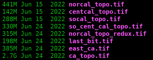
gdal_merge.py -o ca_topo.tif norcal_topo.tif centcal_topo.tif socal_topo.tif so_cent_cal_topo.tif norcal_topo_redux.tif last_bit.tif east_ca.tif

This produced a file called ca_topo.tif. It was very large, in every sense:

^{_{last_little_piece_i_swear_final_final2.tif}}

Using another tool called gdalinfo, we can examine the metadata of the mosaic we just created:

$ gdalinfo -mm ca_topo.tif
Driver: GTiff/GeoTIFF
Files: ca_topo.tif
Size is 40757, 35418
Coordinate System is:
GEOGCRS["WGS 84",
    DATUM["World Geodetic System 1984",
        ELLIPSOID["WGS 84",6378137,298.257223563,
            LENGTHUNIT["metre",1]]],
    PRIMEM["Greenwich",0,
        ANGLEUNIT["degree",0.0174532925199433]],
    CS[ellipsoidal,2],
        AXIS["geodetic latitude (Lat)",north,
            ORDER[1],
            ANGLEUNIT["degree",0.0174532925199433]],
        AXIS["geodetic longitude (Lon)",east,
            ORDER[2],
            ANGLEUNIT["degree",0.0174532925199433]],
    ID["EPSG",4326]]
Data axis to CRS axis mapping: 2,1
Origin = (-125.109583333326071,42.114305555553187)
Pixel Size = (0.000277777777778,-0.000277777777778)
Metadata:
  AREA_OR_POINT=Area
Image Structure Metadata:
  INTERLEAVE=BAND
Corner Coordinates:
Upper Left  (-125.1095833,  42.1143056) (125d 6'34.50"W, 42d 6'51.50"N)
Lower Left  (-125.1095833,  32.2759722) (125d 6'34.50"W, 32d16'33.50"N)
Upper Right (-113.7881944,  42.1143056) (113d47'17.50"W, 42d 6'51.50"N)
Lower Right (-113.7881944,  32.2759722) (113d47'17.50"W, 32d16'33.50"N)
Center      (-119.4488889,  37.1951389) (119d26'56.00"W, 37d11'42.50"N)
Band 1 Block=40757x1 Type=Int16, ColorInterp=Gray
    Computed Min/Max=-130.000,4412.000

If I may draw your attention to a couple things there, the image is 40,757 pixels wide and 35,418 pixels tall. The "pixel size" is 0.000277777777778 by 0.000277777777778; the units, given by the "angleunit", is degrees; 1 arc second is 1/3600th of a degree, which is 0.01754... They're degrees of arc along the surface of the Earth⁵, at a distance measured from the center of the planet. As previously mentioned, that translates into a size of roughly 30 meters. So if you were ever curious about how many 100-ish-foot squares you'd need to fill a rectangle that fully enclosed the entire border of California, then one billion, four-hundred-forty-three million, five-hundred-thirty-one thousand, and four-hundred-twenty-six (40,757 times 35,418) is pretty close.

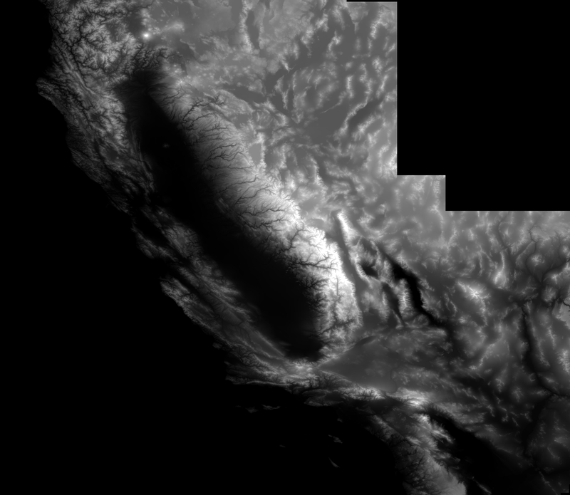
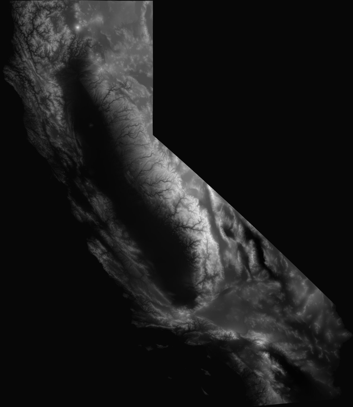
The other units in there are under the "Coordinate System is" section, and are meters relative to the World Geodetic System 1984 vertical datum (distances from this reference surface in the dataset are within 16 meters of the true distance in reality); the very last line is the lowest and highest points in file, which are -130 meters and 4,412 meters respectively, relative to the baseline height defined by the WGS84 ellipsoid. If you were to view the file with an image viewer, it would look like this:

^{_{if you squint, you can kinda see the mountains}}

It's almost completely black because the highest possible value an image like that could have for a pixel is 65,535⁶, and the highest point in our dataset is only 4,412, which is not that much in comparison. Plus, it includes portions of not-California in the height data, and ideally, we want those places to not be represented in our dataset; we have a little more processing to do before we can use this.

Cartography is complicated

The first order of business is to mask out everything that's not California, and the first thing I needed for that was a shapefile that described the California state border. Luckily, that exact thing is publicly available from the state's website; thank you, State of California!

There was only one issue: the shapefile was in a different map projection than the data in our geotiff file. A "map projection" is just the term for how you display a curved, 3D shape (like the border of a state on the curved surface of the Earth) on a flat, 2D surface, like a map. If you look at the line in the output of gdalinfo above that says, ID["EPSG",4326], that is telling us the particular projection used. EPSG 4326 uses latitude and longitude, expressed in degrees, covers the entire Earth including the poles, and references the WGS84 ellipsoid as the ground truth.

The shapefile was in a projection called EPSG 3857, or "Web Mercator". This is similar to EPSG 4326, except instead of using the WGS84 ellipsoid, it pretends the Earth is a perfect sphere. It only covers +/- 85-ish degrees of latitude (so not the poles), and it uses meters instead of degrees of lat/long. It's popular with online map services (like Google Maps and Open Street Maps) for displaying maps, hence the name, "Web Mercator", so you'd probably recognize the shapes of things in it.

Once again, there's a handy GDAL tool, gdalwarp, which is for reprojecting geotiffs. So all we have to do is take our 4326-projected geotiff, use gdalwarp to project it to 3857/Web Mercator, and then we can use the shapefile to mask off all other height data outside the border of California.

It's almost too easy.

gdalwarp -t_srs EPSG:3857 ca_topo.tif ca_topo_mercator.tif

This gives us a 3857-projected file called ca_topo_mercator.tif. It still has over a billion pixels in it (it's a little bigger overall, but the aspect is much wider, with the different projection); scaling it down will be a very last step, since at that point, it will no longer be a digital elevation map, it will just be an image. We'll get there, just not yet.

Cracking open gdalinfo, we get:

$ gdalinfo ca_topo_mercator.tif                             
Driver: GTiff/GeoTIFF
Files: ca_topo_mercator.tif
Size is 36434, 39852
Coordinate System is:
PROJCRS["WGS 84 / Pseudo-Mercator",
    BASEGEOGCRS["WGS 84",
        ENSEMBLE["World Geodetic System 1984 ensemble",
            MEMBER["World Geodetic System 1984 (Transit)"],
            MEMBER["World Geodetic System 1984 (G730)"],
            MEMBER["World Geodetic System 1984 (G873)"],
            MEMBER["World Geodetic System 1984 (G1150)"],
            MEMBER["World Geodetic System 1984 (G1674)"],
            MEMBER["World Geodetic System 1984 (G1762)"],
            MEMBER["World Geodetic System 1984 (G2139)"],
            ELLIPSOID["WGS 84",6378137,298.257223563,
                LENGTHUNIT["metre",1]],
            ENSEMBLEACCURACY[2.0]],
        PRIMEM["Greenwich",0,
            ANGLEUNIT["degree",0.0174532925199433]],
        ID["EPSG",4326]],
    CONVERSION["Popular Visualisation Pseudo-Mercator",
        METHOD["Popular Visualisation Pseudo Mercator",
            ID["EPSG",1024]],
        PARAMETER["Latitude of natural origin",0,
            ANGLEUNIT["degree",0.0174532925199433],
            ID["EPSG",8801]],
        PARAMETER["Longitude of natural origin",0,
            ANGLEUNIT["degree",0.0174532925199433],
            ID["EPSG",8802]],
        PARAMETER["False easting",0,
            LENGTHUNIT["metre",1],
            ID["EPSG",8806]],
        PARAMETER["False northing",0,
            LENGTHUNIT["metre",1],
            ID["EPSG",8807]]],
    CS[Cartesian,2],
        AXIS["easting (X)",east,
            ORDER[1],
            LENGTHUNIT["metre",1]],
        AXIS["northing (Y)",north,
            ORDER[2],
            LENGTHUNIT["metre",1]],
    USAGE[
        SCOPE["Web mapping and visualisation."],
        AREA["World between 85.06°S and 85.06°N."],
        BBOX[-85.06,-180,85.06,180]],
    ID["EPSG",3857]]
Data axis to CRS axis mapping: 1,2
Origin = (-13927135.110024485737085,5178117.270359318703413)
Pixel Size = (34.591411839078859,-34.591411839078859)
Metadata:
  AREA_OR_POINT=Area
Image Structure Metadata:
  INTERLEAVE=BAND
Corner Coordinates:
Upper Left  (-13927135.110, 5178117.270) (125d 6'34.50"W, 42d 6'51.50"N)
Lower Left  (-13927135.110, 3799580.326) (125d 6'34.50"W, 32d16'33.21"N)
Upper Right (-12666831.611, 5178117.270) (113d47'17.10"W, 42d 6'51.50"N)
Lower Right (-12666831.611, 3799580.326) (113d47'17.10"W, 32d16'33.21"N)
Center      (-13296983.361, 4488848.798) (119d26'55.80"W, 37d21'21.69"N)
Band 1 Block=36434x1 Type=Int16, ColorInterp=Gray

You can see that the PROJCRS[ID] value is "EPSG,3857", as expected. The "pixel size" is "34.591411...." and the "lengthunit" is "metre". But the number of pixels is different, and the shape is different, yet the coordinates of the bounding corners are the same as the original file's (the latitude and longitude given as the second tuple). This is all from the Web Mercator's different projection causing the aspect ratio to stretch horizontally, but it still represents the same area of the planet.

The one custom script

Now that we had our geotiff in the right projection, the next step was use the shapefile to mask out the California border in it. Here is where GDAL failed me, and looking around now as I write this, I still can't find a specific GDAL tool for doing it. Given how useful I found all the other tools, I can't really complain, so I won't! It wasn't that hard to write something that would do it with other open source tools; I didn't even bother checking this into a git repo or anything:

#!/usr/bin/env python3

import fiona                  # for reading the shapefile
import rasterio               # for working with the geotiff
import rasterio.mask as rmask

import sys

def main():
    tif = sys.argv[1]
    msk = sys.argv[2]
    out = sys.argv[3]

    print("input: {tif}\nmask: {msk}\noutput: {out}".format(tif=tif, msk=msk, out=out))
    if input("Enter 'y' to continue: ").lower() != 'y': # double-check I don't stomp something I wanted to keep
        print("See ya.")
        return

    with fiona.open(msk, "r") as shapefile:
        shapes = [feature["geometry"] for feature in shapefile]

        with rasterio.open(tif) as in_tif:
            out_image, out_xform = rmask.mask(in_tif, shapes, filled=True, crop=True)
            out_meta = in_tif.meta
            out_meta.update({"driver": "GTiff",
                             "height": out_image.shape[1],
                             "width": out_image.shape[2],
                             "transform": out_xform})
            for k, v in out_meta.items():
                print("{}: {}".format(k, v)) # just outta curiosity

            with rasterio.open(out, "w", **out_meta) as dest:
                dest.write(out_image)

    print("Wrote masked tif to {}".format(out))

    return

if __name__ == "__main__":
    main()

I include that just in case anyone else ever needs to do this, and doesn't find one of the hundreds of other examples out there already. This one is nice because you don't need to pre-process the shapefile into GeoJSON or anything, the Fiona package handles things like that transparently for you, but don't think this is great Python or anything; it's the dumbest, quickest thing I could crap out to do the task I needed to be done⁷.

After running that script, I had a Web Mercator-projected geotiff that included data only for places inside the state border of California. It was still enormous; the mask didn't change the shape and you can't have non-rectangular images anyway, but at this point, I had the final desired dataset. It was time to turn it into a heightmap that we could use to make a mesh.

A usable heightmap

I've been trying to be careful about referring to the image file as a "dataset" or "geotiff", vs. a "heightmap". A geotiff file is not a regular image file, it includes particular metadata and data that is meant to be interpreted as a real map of the land; each pixel in it says something about an exact, actual location in the real world. In our geotiff, a mountain would have to be more than twelve miles high before it appeared as bright white⁸.

A "heightmap" is an image file, like a geotiff, where each pixel's monochromatic intensity is meant to represent height above some lowest plane. The difference is that the height values are normalized so that the lowest height is 0, and the highest is the maximum possible value in the format's value range. For geotiff digital elevation maps, which use 16-bit numbers as previously mentioned, that maximum possible value is 65,535. But unlike a geotiff, a generic heightmap has no exact correspondence with anything else; it's not necessarily an accurate dataset, and won't include the GIS stuff like what projection it is, what the coordinate bounding boxes are, etc. But it is useful for turning into a mesh.

And here I get to the final GDAL tool I used, gdal_translate. This is something that can read in a geotiff, and write out a different image format. When in doubt, PNG is fine, I always say. It's a simple format that nearly everything can read, and is compressed so it should be a much smaller file on disk, even if it's the same number of pixels. Smaller file size is always easier.

gdal_translate -of PNG -ot UInt16 -scale -130 4412 0 65535 masked_ca_topo.tif heightmap.png

Like we saw earlier, the lowest point we had in our data was -130 meters, and the highest was 4,412. The -scale -130 4412 0 65535 arguments are saying, "anything with a height of -130 should be totally dark, and anything with a height of 4,412 should be as bright as possible, and anything in-between should be set proportionately." This is a linear mapping, and preserves the relationships between vertical features (that is, if something is twice as tall as another thing, that will still be true after being scaled), so in a sense, it's "accurate", but would it be good, was the question (note: more foreshadowing).

Once I had the PNG file, I used the ImageMagick convert command to resize the file down to a reasonable size. Finally, I had something I could use to make a mesh:

Pretty cool, right? I thought so! The detail is pretty great; that bright spot near the top is Mt. Shasta, for example; Mt. Whitney is slightly taller, but not by much, and is part of a range so it doesn't stand out the way Shasta does. It was time to start making some 3D geometry with the heightmap⁹!

A mesh is born

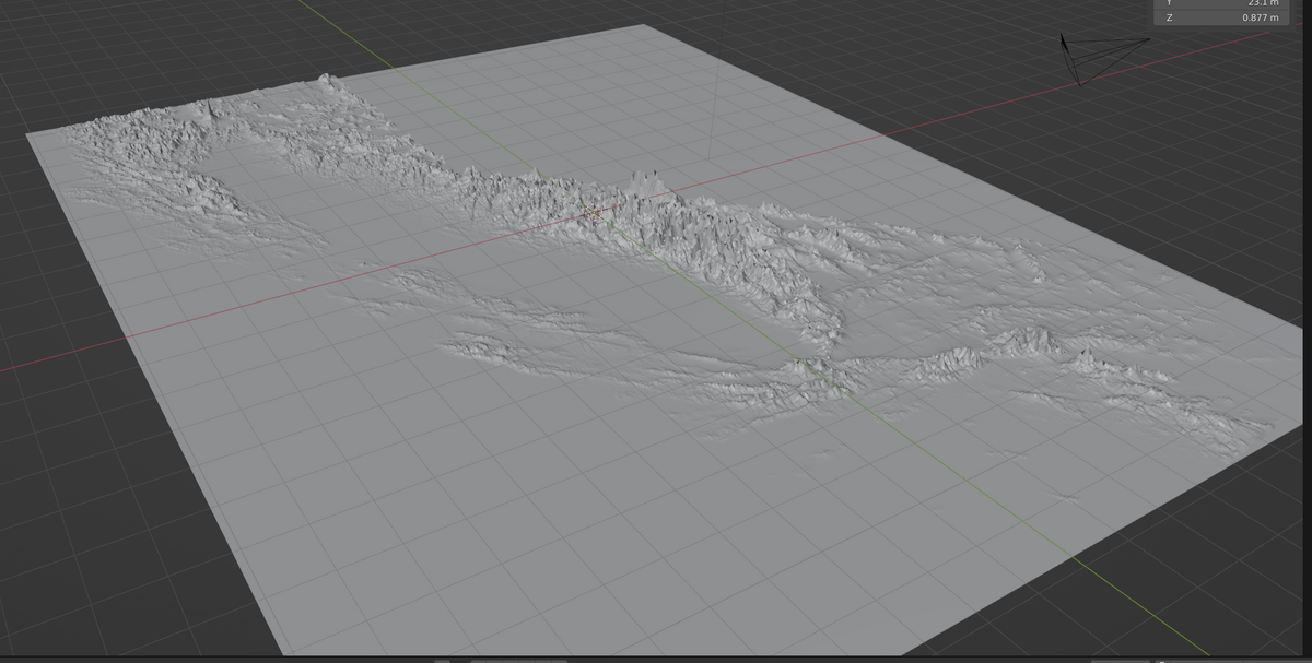
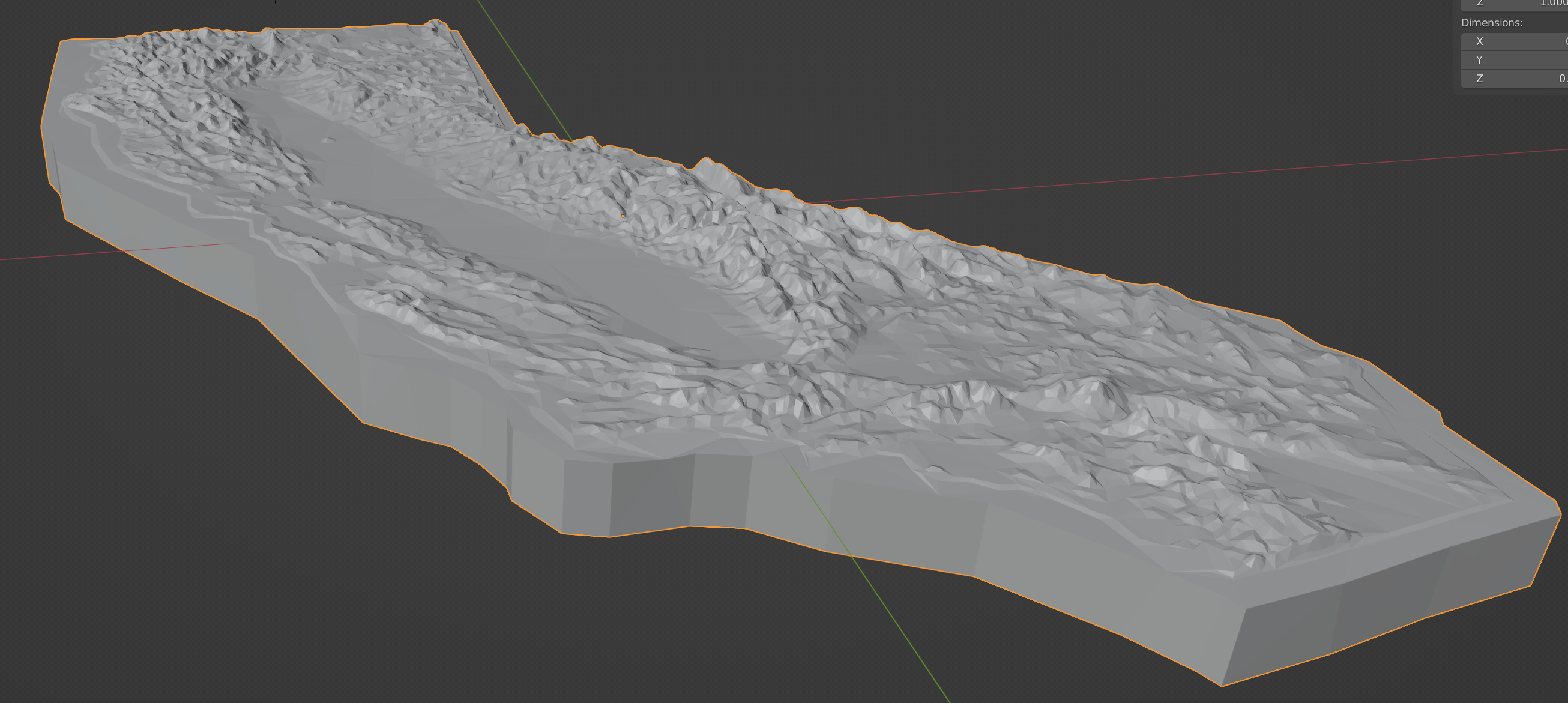
My next step was to figure out how exactly to turn that heightmap into a mesh. Some searching assured me that Blender, a free and open source 3D modeling package that I'd dabbled with before, would work well. For example, here's a pretty high-level walk-through of how to use a heightmap to displace a mesh plane, which is almost exactly what I first wanted to do. Before too long, I had something that looked like this:

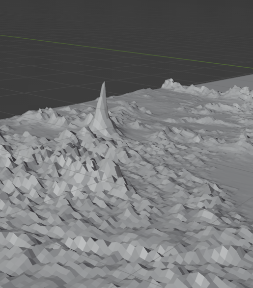
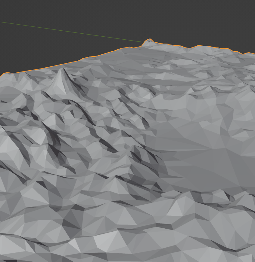
At first glance, it looks OK, but there's so. much. detail. And it's very, very pointy; it just looks jagged. Check out this close-up detail of Mt. Shasta:

^{_{witch's hat-assed mountain}}

You can tell it wounldn't be nice to touch, and being able to run your fingers along the shape was a huge part of the appeal of having the physical object.

Back to the realm of images

Given that it seemed like there were at least a couple semi-related problems from too much detail, my first instinct was to blur the heightmap, and then reduce the size of it. I used the ImageMagick convert command again to blur the image a couple rounds, and then resized it down:

A little better, but still not great. A few more rounds of blurring and shrinking got me this:

With that version, I was able to produce some reasonable-looking geometry in Blender:

Or so I thought.

It may have been smoother, it was still very pointy. A lot of the high-frequency detail has been removed, which means it's not rough and jagged, but Shasta still looks ridiculous.

A matter of scale

The problem was that I was doing a linear scaling of the height of features in the data, and the required factors were so enormous that it distorted the geometry in an ugly way.

The State of California is very large, but for the sake of argument, let's pretend it's exactly 700 miles tall, from the southern tip to the northern border's latitude, going straight north; the real length is close to that. Also for the sake of argument, let's say that the tallest mountain is 3 miles tall; the actual height is a little less than that, but that's OK, the argument holds more strongly at lower height. That means the ratio of height to length is 3/700, or 0.0043-ish.

If you had a physically accurate topographic carving of California that was a foot long, the tallest peak on the carving would be 0.0043 feet high, which is about 1/20th of an inch, or about 1.3 millimeters. You'd probably be able to see and feel where Shasta was, and see that there was a faint line from the Sierra Nevadas, but that would be it. That's why it's so hard to see the details in the raw elevation data geotiff.

In order to be able to see any detail, and to meet expectations about what a topographic carving is supposed to look like, the height of the highest peaks needs to be scaled up by something like 10-20x. My problem was that I was doing a linear scale; I was making everything 10-20x taller than it "should" be, which was causing everything to look stretched and weird.

And even with that amount of exaggeration, some low-elevation features were still not showing up. For example, Sutter Buttes, a 2,000-foot tall mound in the Sacramento Valley, which is faintly visible in the heightmap, is almost not there in the resulting mesh. It's about 1/7th the height of Shasta, which is not all that much, when Shasta was represented by something 0.75 inches tall.

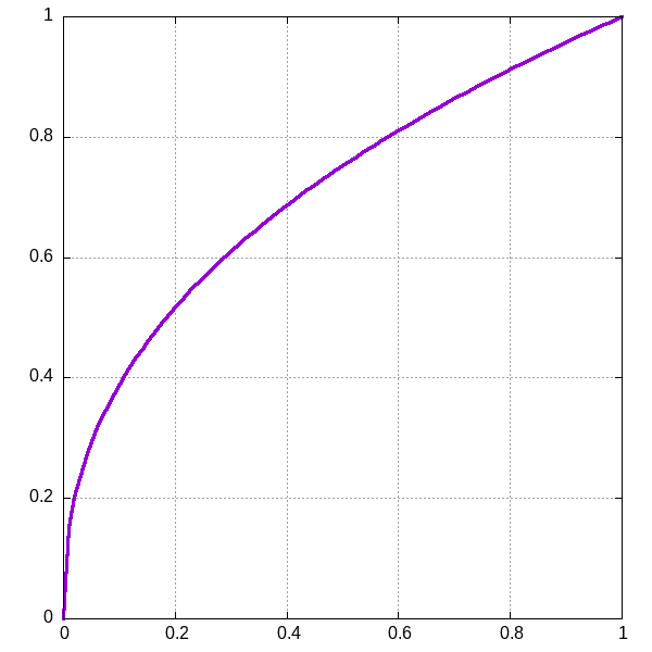
What I really needed was some non-linear way to scale the height, some way to exaggerate lower altitudes more than higher ones. The highest points should stay as high as they were; they determine the ultimate overall height, but lower points should be given a relative boost. An easy way to do this is to take some fractional root (raise a number to a power between 0.0 and 1.0) of the linear scaling factor, and use that new value instead. For example, the graph of x raised to the 0.41th¹⁰ power looks like this:

Notice how values at 0 and 1 are the same as they would be with linear scaling, values near 0 rapidly get scaled upward, and by the time you get near 1, it looks almost linear again. The linear scaling function we'd initially used would just look like a straight line from the lower left corner to the upper right.

Luckily, gdal_translate has an option to do this kind of scaling, so it was a quick

gdal_translate -of PNG -ot UInt16 -scale -130 4412 0 65535 -exponent 0.41 ca_topo.tif exponentially_scaled_heightmap.png

and a couple rounds of blurring, and I had the following heightmap:

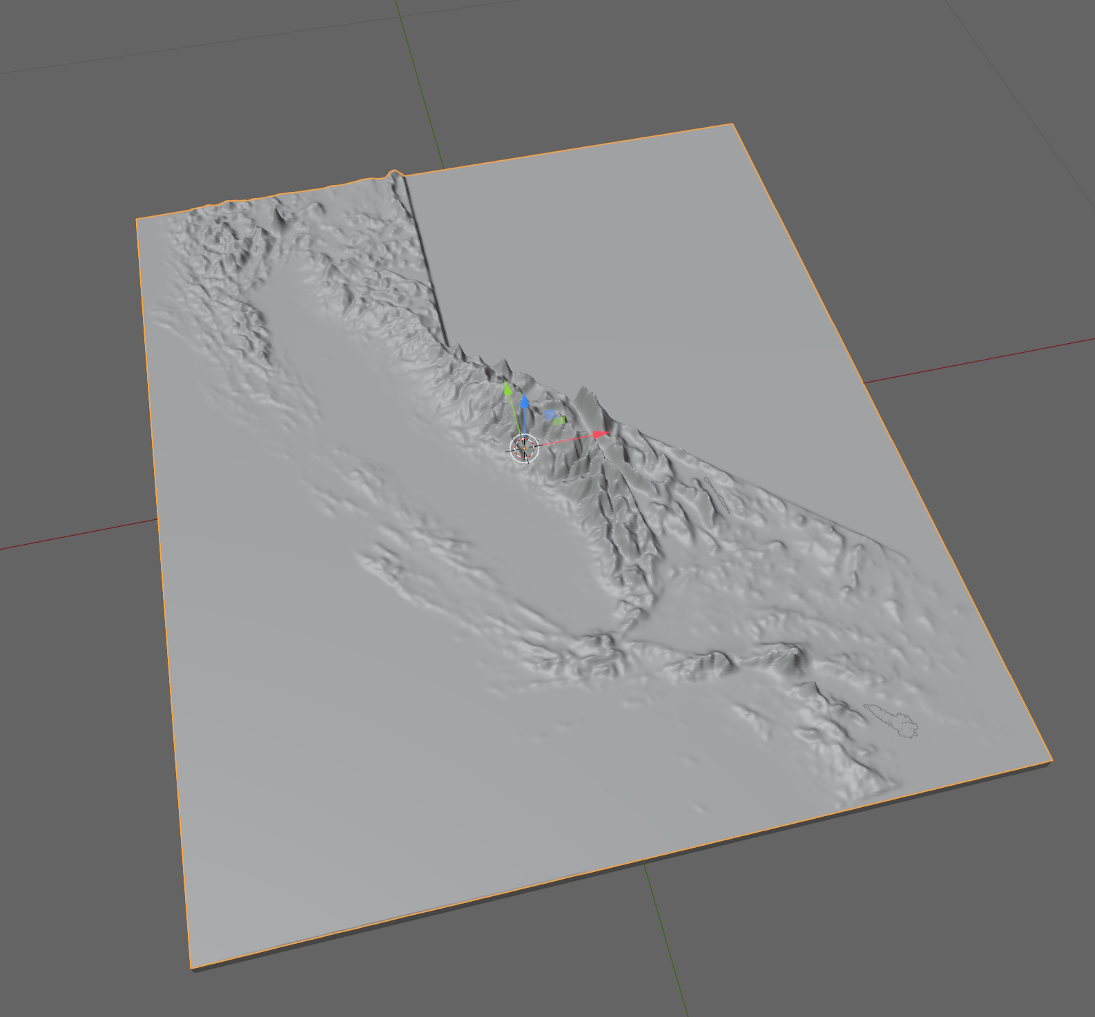
which resulted in a mesh that looked something like this inside Blender:

Doesn't that look nicer? Notice how a bunch of things that were nearly invisible before, like Sutter Buttes, are easily visible. Check out the Channel Islands now plain as day! I was feeling pretty good about having this whole thing wrapped up shortly, only a little late for the birthday.

A dark age

What followed was two frustrating weeks attempting to get a manifold mesh out of Blender that was small enough, by which I mean number of vertices and edges, so that FreeCAD could turn it into an STP file. Unfortunately, FreeCAD is not a good tool for doing fancy things with meshes, like creating them from a heightmap, so I had to use two different tools.

This also meant that I would run into surprising limits when going between them. Let me explain. I'd get a mesh in Blender, export it to a neutral mesh format like OBJ that both programs understand well, and it would be a 60 megabyte file. My computer has 32 gigabytes, more than 500 times more memory than that, so you'd think it would not be a problem.

The act of asking FreeCAD to import that OBJ file as a mesh, and not even as a solid body, caused the memory use to go to 21 gigabytes. This is a lot, but the computer still had plenty of room left in memory for things like "responding to the keyboard and mouse" or "redrawing the screen". Everything at this point is still perfectly usable.

When I attempted to convert that mesh into a solid body, though, memory use ballooned up to encompass all available RAM, and my system immediately came to a nearly imperceptible crawl until my frantic ctrl-cs were finally registered by the signal handlers in FreeCAD before I could use it again. This happened a lot. At last, the prophecy had come to pass.

I went through many rounds of attempting to clean up the mesh and reduce its complexity, but I don't have many notes or intermediate artifacts from this time. A lot of that was being a beginner at both Blender and FreeCAD, though there's so much educational material that I was rarely held back by not knowing how to do a particular thing inside each program. A lot was inexperience in the domain; I did not know how much detail was essential, and I did not have a lot of experience with digital modeling in the first place. The workflow was very manual, and cycles were fairly long, which made it hard to try a bunch of things in quick succession as experiments. All those things and more conspired to make this portion of the process a total slog with very little to show off.

Test prints

Eventually, after a couple weeks of trying and failing to get something into FreeCAD that I could then work with (like merging it with a thick base and trimming that base to follow the shape of the state), I had had enough. I was just going to send the shop an STL file and forget about trying to get an STP file. I have some notes from then, right after I'd started my first test print:

I'm finally printing something out. I've given up on converting it into [something CAD-friendly]; it seems this is a Hard Problem, but I'm not sure why. My goal with doing that was to give a CAD-friendly file to a local CNC milling shop, per their request, since when I suggested a mesh-based file (STL), the guy was like "I can't do much manipulation with that to make it more manufacturable, so a real CAD file would be best".

But at least with an STL file, I can print it myself. So that's going now, we'll see how it turns out in no less than eight hours.

I haven't really done anything else with my computer besides this for a while.

When that print was done, here's what it looked like:

^{_{don't look at me, I'm hideous}}

In case you were not revolted enough, then please allow me to direct your gaze toward this eldritch abomination:

^{_{what did I just say about looking at me}}

As bad as it looked, it felt even worse to touch. Setting aside the hideous base with its weird visual artifacts due to those areas not being a single flat polygon, but rather several polygons that were not parallel, there was still just too much high-frequency detail in the terrain, and it was a total mismatch with the 3D printed medium.

The real thing was going to be carved out of wood by a CNC mill, which uses a drill-like component to carve away pieces of the material you're working with. This means that there's a tiny spinning bit with a definite, finite size, and any detail in the model smaller than the end of that spinning bit would likely be impossible to carve with it. This meant that all that high-frequency detail was not only ugly, it was also completely unnecessary.

Just try harder

I was very eager to get something into the CNC shop's hands at this point, but I also knew that this model was not acceptable. So, I resolved to brutally simplify the geometry until I got something that was workable inside FreeCAD.

First off, I made the heightmap even smaller, only 500 pixels wide. Fewer pixels means fewer details for turning into a displacement map for a mesh! I also removed the Channel Islands from the heightmap, resulting in this final mesh displacement input:

^{_{it's the final heightmap (doot-doot-doot-doot,
doot-doot-doot-doot-doot)}}

Inside Blender, I'd gotten quite proficient at running through the steps to generate a mesh from a heightmap, and once I'd done that, I went through several rounds of mesh simplification; the geometry was practically homeopathic.

^{_{by the principles of homeopathy, the fewer the vertices, the more potent the mesh}}

Check out this close-up of Mt Shasta:

^{_{a chonkier, less lonesome Mt Shasta}}

Present, but not obnoxious. I printed out a second test print to make sure it looked as good in physical reality:

Verdict: yes. If you want, you can visit https://www.printables.com/model/240867-topographic-california and download the 3D printer file to print it yourself at home. If you don't have a 3D printer, you can still look at and interact with a 3D model of it in the browser on that site, so it's still kind of neat. A couple different strangers uploaded pictures of their prints of it, which I thought was cool!

I brought the mesh into FreeCAD and finally was able to create the STP¹¹ file the shop had asked for, a mere twenty-five days after I'd last spoken with them.

Final cut

I emailed the file to the shop, and said,

As modeled, there's probably more high-frequency detail in the mountains than is necessary, as I'm going for something that feels nice to the touch so smoother is better. It's also modeled at a slightly larger scale than necessary, though not too far off (it's 500x577mm, and I'm interested in the 400-500mm range for width; the relief height is in the 20-30mm range depending on scale). I was imagining it would be carved with contour cuts in some thick nice ply, though I'm happy to hear better ideas; I have literally no experience with making something like this.

The shop came back with,

I can’t smooth out the cuts, I can only cut what is there. That being said, if I use a rounded cutter, it will round out the valleys but not the peaks as it won’t go into areas that it can’t reach.

Hope that makes sense.

Let me know if this will work for you or not. If you think it will, I will try to program the toolpaths and see what it will look like.

I definitely didn't want to lose the sharp seams in the bottoms of the valleys!

Me: I guess what I was really saying is that if some detail is lost due to using a larger cutting head that's probably fine. I wouldn't necessarily want the valleys to be made more concave than they already are, though. Does that make sense?

Shop: Yes, that makes sense. I can use a Vee cutter and it will cut the sharp edges in the valleys."

It felt nice to be understood! Next came the issue of cost:

I ran the numbers on both sizes using a .01” step-over cut, meaning that is how far apart the finish cuts will be from each other.

You will probably see some tool marks depending on what type of material is used.

The larger one is coming in at around $850.00 and the 12” one at $350.00.

I can go tighter, say .005” step-over and it will probably not show many marks but I won’t know until I run it.

If I do that it will double the cut time so close to doubling the price.

One of the things that my wife had said she wanted to do with the carving of California was sand and finish it herself, so the coarser 0.01-inch step-over cut was not really a problem. Even the 0.005-inch cut would still require a final sanding before staining or sealing.

The "larger one" the shop referred to was for a 20-inch wide carving, which would be way too huge anyway; 12 inches was fine. Still, $350 was at the top of what I had hoped/expected to spend. I hoped it was worth it!

After a few more back-and-forths and days, I got a message from the shop saying it was ready. They also said,

I decided to run these with half the original step-over, which means it takes twice as long but the finish is almost smooth. I think you will be pleased with it.

Whoa! This meant he had used the 0.005-inch cutting resolution, and the job had taken twice as long as originally quoted. Like the kind and generous tailor from The Hudsucker Proxy, he had given me the double-stitch anyway, even though I had insisted that single stitch was fine. I was very excited and grateful, and couldn't wait to see it.

Pics or it didn't happen

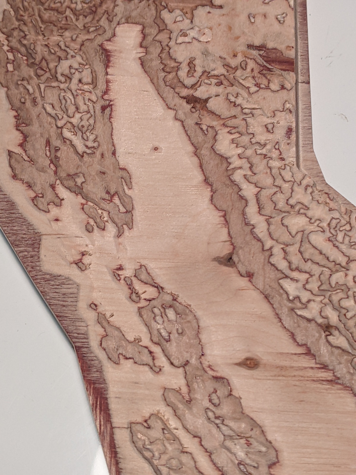
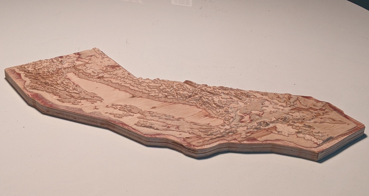
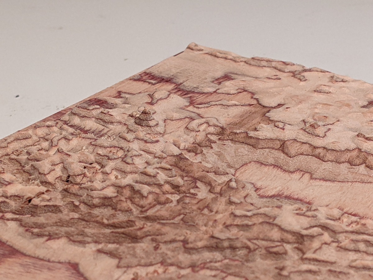
When I got there, it was almost exactly what I had imagined and hoped it would be. Obviously, you've seen the photo at the top of the page, but please enjoy this CNC-carved topographic California porn.

^{_{some nice soft lighting}}

^{_{sutter buttes, we meet again}}

^{_{recognize this angle, from blender?}}

^{_{lookin' good, shasta}}

I wasn't the only one pleased with it; my wife was delighted when she saw it.

MISSION ACCOMPLISHED, HAPPY _belated BIRTHDAY!

Thank yous

Obviously, I have tons of people to thank for their help with this, either directly or indirectly. First and foremost, my wife, for everything, but especially for the inspiration and also patience with me during this process.

A close second for this project goes to Steve at Triumph CNC. He asked me what I was going to do with it, and when I said give it to my wife as a gift, he said, "Oh, that's great! I feel even better about using the smaller step-over now." If you need some CNC milling done in Los Angeles, maybe give them a call!

Along the way during this journey I got a lot of feedback and suggestions from friends and colleagues, so thank you, 'rades¹²!

Of course, this would all have been unthinkably difficult not so long ago, but thanks to things like NASA's missions and public GIS datasets, almost anyone can do something like this.

And not just public, government data and organizations, but private, passion-driven free software projects like Blender and FreeCAD that rival functionality found in multi-thousand-dollar commercial packages. I'm in awe of their accomplishments; they are true wonders of the modern world.

Things I learned, and some lessons

I said early on that I knew basically nothing about any of this, and that was true. I had had some earlier casual experience with both Blender and FreeCAD, and many, many years ago I had taken a semester of engineering drafting my first year of college. But I knew basically nothing about GIS, about the different map projections, about shapefiles, about any of the tools or jargon. Likewise, I have no experience or instruction in any kind of CNC milling; my scant 3D printing experience doesn't really apply.

This article is as close as I could get to serializing nearly everything I had to learn and do to create that carving.

And at the time it was happening, it didn't feel like I was retaining all of it, or that I really, truly understood everything I had done; I was hurrying as fast as I could toward a particular goal. But in the course of writing this, I was basically retracing my steps, and found that I really did have a pretty good handle on it. One of my favorite things to do is learn stuff, so this was a great outcome for me!

If I were to do this again, or if I were starting for the first time with the benefit of someone else's experience, there are obviously a few things I would do differently. First off, I'd see if I could find a lower-resolution dataset. One arc second is way overkill; at the scale of a topo carving that you can hold in your hands, a resolution of several arc minutes (one arc minute is one nautical mile, which is about 1.1 regular (terrestrial?) miles) would probably be enough.

I'd also use the USGS national map downloader site to get just the California data; you can upload a shapefile and it'll give you back a masked geotiff. If I had started from that, it would have shaved at least two weeks off the time it took me to make the thing; I could have jumped immediately into being frustrated in Blender and FreeCAD.

Speaking of, I wish I could give some guidance on effectively using Blender and FreeCAD, but that's a journey only you can plot. That's probably not true, but I still feel like a doofus in those tools, so I don't feel like it's worth anyone's time to hear from me about them. Good luck in your quest!

The conclusion upon examination was, "I just wasn't thinking". ↩︎
I'm pretty sure this is more "represent shapes with math" than with a computer, but the computer is helping us do the math and it's more relatable. ↩︎
I think you could also have a 2D sheet with a hole cut out of it represented by a mesh that is manifold, as long as the connectivity was correct in terms of how many shared edges and vertices there were (though this would not be a valid STL file). Imagine a cloth sheet with a hole cut out in the middle, and the edge of the hole hemmed or otherwise "sealed", which is then a manifold boundary. See this powerpoint deck for a pretty math-y overview of "mesh basics" (but not really that basic, that's just academics trolling us, don't let it bother you). If I'm wrong about a 2D sheet with a hole being possibly manifold, I invite correction! ↩︎
A textbook example of Chekhov's Scarce Computational Resource. ↩︎
Technically, it's an arc along the WGS84 ellipsoid, which is a perfectly smooth smushed sphere, which more closely matches the real shape of the Earth vs. a perfectly round sphere. ↩︎
Each pixel is 16 bits, so the possible values are from 0 to 2^16 - 1. 2^16 is 65536, so there you go. ↩︎
A friend posited at one point that my circuitous journey to the end product was the point, but I assured him that every step I took was trying to get to the end product as quickly and straightforwardly as possible. Still, I did in fact wind up learning a whole shitload of stuff, which is nice, I GUESS. ↩︎
I'm not actually sure what the "0" altitude pixel value is. It can't actually be 0, because the numbers in the file can't be negative, and there are deep valleys on the earth's surface. But it's clearly not that high a value, otherwise, when you viewed the geotiff as an image, it would be closer to white or gray than black. ↩︎
Based on the timestamps of the files in the directory where I was working on this project, it took about ten days from the time I first downloaded a geotiff dataset to having the heightmap shown above, so you can imagine all the dead-ends I went down and did not share in this write-up. ↩︎
I think this was just the first fractional value that I tried, and it was fine. ↩︎
I actually produced an IGES file; STP is basically fancy IGES, and my model didn't include the extra info in STP files like material and color anyway. ↩︎
pronounced "rads", and is short for "comrades". ↩︎

48 KiB Raw Blame History Unescape Escape