15 KiB

Raw Blame History

+++ title = "A Thoroughly Digital Artifact" slug = "a-thoroughly-digital-artifact" date = "2023-01-11" [taxonomies] tags = ["3dprinting", "CAD", "GIS", "CNC", "art", "sundries", "proclamation"] +++

A birthday wish

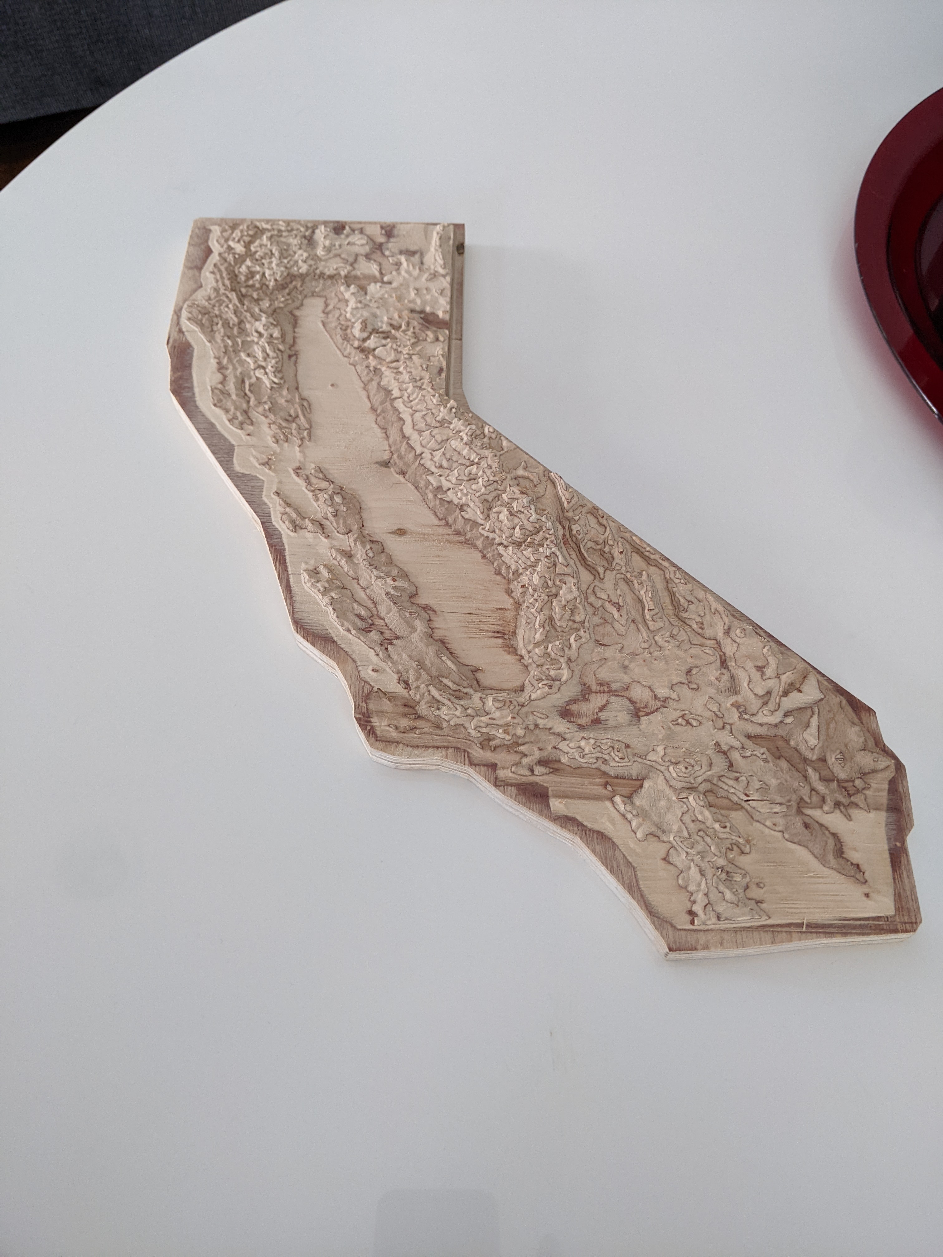
Last summer, I wanted to get my wife something nice for her birthday. For many years, she had expressed an occasional and casual desire for a topographic carving of the state of California, where we live, and I thought it might be something I could figure out how to get her. In the end, after many dozens of hours of work, five weeks, and several hundred dollars paid to a professional CNC machine shop, I had the artifact shown in the picture above. This is the story of its creation.

First steps

Before you ask, I did not do a ton of research before embarking on this. As I write this, about six months later, it only now occurred to me to do a basic search for an actual physical thing I could buy, and luckily it seems that CNC-carved wooden relief maps of the whole state are not trivially easy to come by, so, phew!

No, my first step was to see if there were any shops in the area that could carve something out of nice plywood, about a week before the intended recipient's birthday. I found one that was less than ten minutes away, and filled out their web contact form. They had a field for material, and I said, "some nice plywood between 0.75 and 1.0 inches thick or similar" (I didn't know exactly what was available and wanted to give broad acceptable parameters), and under "project description", I wrote,

A relief map of California, carved from wood. Height exaggerated enough to visibly discern the Santa Monica mountains. I can provide an STL file if needed.

For some [incorrect] reason that I only later examined, I just sort of assumed that the shop would have a library of shapes available for instantiating into whatever material medium you might need. But just in case, I included that hedge about being able to provide an STL file. Needless to say, that was a bluff.

^{_{me, every single time}}

Also needless to say, my bluff was immediately called, and I had the following exchange with the shop:

CNC Shop: STL can work but I can’t manipulate it, which could save some money. If possible can it be exported to an .igs or .iges or .stp format?

Me: Yeah, STP should be no problem. Can you give a rough estimate of the cost for 1x2-foot relief carving?

Shop: Without seeing the drawings, I can’t give even a close price but in the past they range from a few hundred dollars to several thousand dollars.

Me: That's totally fair! I'll get you some files in a few days.

"STP should be no problem ... I'll get you some files in a few days," was an even harder lean into the bluff; my next communication with the shop was nearly four weeks later. But that's getting ahead of things.

Meshes and solid bodies

First off, let's talk about file formats and how to represent shapes with a computer.¹ I first said I could provide an STL file. STL is a pretty bare-bones format that describes the outside surface of a shape as a mesh of many, many triangles, each of which is described by three 3D points, where each point (but not necessarily each edge) of the triangle lies on the surface of the shape of the thing you're modeling. This format is popular with 3D printers, which is how I became familiar with it.

STL is simple to implement and easy for a computer to read, but if you have a model in that format that you need to manipulate, like you want to merge it with another shape, you won't have a good time. In order to actually do things like change the shape of the model, it needs to be converted into a CAD program's native representation of a "solid body", which is pretty much what it sounds like: a shape made of a finite volume of "stuff", and NOT just an infinitesimally thin shell enclosing an empty volume, which is what the STL mesh is.

In order for the CAD program to convert a mesh into a solid body, the mesh must be manifold, meaning, no missing faces (triangles), and with a clearly-defined interior and exterior (all triangles are facing in one direction relative to their interior). When there are no missing faces, it's called "water tight". You can still have "holes" in a mesh, like if you have a model of a donut², but the surface of the donut can't have any missing faces. A valid STL file's meshes are manifold.

The CNC shop had requested a model in a format called STP. .stp is the extension for a "STEP" file; STEP is supposed to be short for "standard for the exchange of product data", so someone was playing pretty fast and loose with their initialisms, but I digress. The main thing about STEP files is that CAD programs can really easily convert them into their native internal solid body representation, which allows easy manipulation. Another thing about them is that a CAD program can usually turn an STL file into an STP file, unless the mesh is too complicated and your computer doesn't have enough RAM (note: foreshadowing³).

^{_{this cube's mesh has too many vertices and edges, I hope my computer has enough
RAM to work with it}}

But so far, I had nothing at all. Time to get some data and see if I can turn it into a model.

Public data

My first impulse was to search USGS's website for heightmap data, but I wound up not finding anything appropriate. Once again, now that I'm looking after I'm done, I found this, which would have been perfect:

https://apps.nationalmap.gov/downloader/

Did I just accidentally miss it then? Did I not know how to recognize it because I didn't know what I was doing at all? The world may never know, but at least now you can benefit from my many, many missteps.

From space?

Anyway, having not found anything I could really use from the USGS, I found this site, from OpenTopography, an organization run by the UCSD Supercomputer Center, under a grant from the National Science Foundation. So, hooray for public data!

That particular page is for a particular dataset; in this case, "SRTM GL1 Global 30m". "SRTM" stands for "Shuttle Radar Topography Mission", which was a Space Shuttle mission in February, 2000, where it did a fancy radar scan of most of the land on Earth. Though, it's hard to verify that the data was not synthesized with other datasets of more recent, non-space origin, especially in places like California. But probably space was involved in some way.

In Australia, it's pronounced "g'dal"

Anyway, I'd found an open source of public data. This dataset's horizontal resolution is 1 arc second (which is why it's "GL1"), or roughly 30x30 meters, and the height data is accurate to within 16 meters. Not too shabby!

They provided the data in the form of GeoTIFFs, which are basically an image where each pixel represents one data point (so, a 30x30 square meter plot) centered at a particular location on the Earth's surface. It's a monochrome image, where height is mapped to brightness, so the lowest spot's value is 0 (black), and the highest spot is 65535⁴ (brightest white).

The only problem was that you could only download data covering up to 450,000 square kilometers at a time, so I had had to download a bunch of separate files and then mosaic them together. Luckily, there's a whole suite of open source tools called GDAL. Among that suite is a tool called gdal_merge.py (yes, the .py is part of the name of the tool that gets installed to your system when you install the GDAL tools), which does exactly what I wanted:

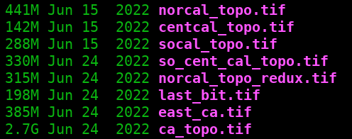
gdal_merge.py -o ca_topo.tif norcal_topo.tif centcal_topo.tif socal_topo.tif so_cent_cal_topo.tif norcal_topo_redux.tif last_bit.tif east_ca.tif

This produced a file called ca_topo.tif. It was very large, in every sense:

^{_{last_little_piece_i_swear_final_final2.tif}}

Using another tool called gdalinfo, we can examine the metadata of the mosaic we just created:

$ gdalinfo -mm ca_topo.tif
Driver: GTiff/GeoTIFF
Files: ca_topo.tif
Size is 40757, 35418
Coordinate System is:
GEOGCRS["WGS 84",
    DATUM["World Geodetic System 1984",
        ELLIPSOID["WGS 84",6378137,298.257223563,
            LENGTHUNIT["metre",1]]],
    PRIMEM["Greenwich",0,
        ANGLEUNIT["degree",0.0174532925199433]],
    CS[ellipsoidal,2],
        AXIS["geodetic latitude (Lat)",north,
            ORDER[1],
            ANGLEUNIT["degree",0.0174532925199433]],
        AXIS["geodetic longitude (Lon)",east,
            ORDER[2],
            ANGLEUNIT["degree",0.0174532925199433]],
    ID["EPSG",4326]]
Data axis to CRS axis mapping: 2,1
Origin = (-125.109583333326071,42.114305555553187)
Pixel Size = (0.000277777777778,-0.000277777777778)
Metadata:
  AREA_OR_POINT=Area
Image Structure Metadata:
  INTERLEAVE=BAND
Corner Coordinates:
Upper Left  (-125.1095833,  42.1143056) (125d 6'34.50"W, 42d 6'51.50"N)
Lower Left  (-125.1095833,  32.2759722) (125d 6'34.50"W, 32d16'33.50"N)
Upper Right (-113.7881944,  42.1143056) (113d47'17.50"W, 42d 6'51.50"N)
Lower Right (-113.7881944,  32.2759722) (113d47'17.50"W, 32d16'33.50"N)
Center      (-119.4488889,  37.1951389) (119d26'56.00"W, 37d11'42.50"N)
Band 1 Block=40757x1 Type=Int16, ColorInterp=Gray
    Computed Min/Max=-130.000,4412.000

If I may draw your attention to a couple things there, that's an image that's 40,757 pixels wide and 35,418 pixels tall. The "pixel size" is 0.000277777777778 by 0.000277777777778; since each pixel is 1 arc second, and 1 arc second is 1/3600th of a degree, and 1/3600 is 0.000277777777..., we can infer that the unit of size there is degrees of arc along the surface of the Earth⁵, at a distance measured from the center of the planet. As previously mentioned, that translates into a size of roughly 30 meters. So if you were ever curious about how many 100-ish-foot squares you'd need to fill a rectangle that fully enclosed the entire border of California, then one billion, four-hundred-forty-three million, five-hundred-thirty-one thousand, and four-hundred-twenty-six (40,757 times 35,418) is pretty close.

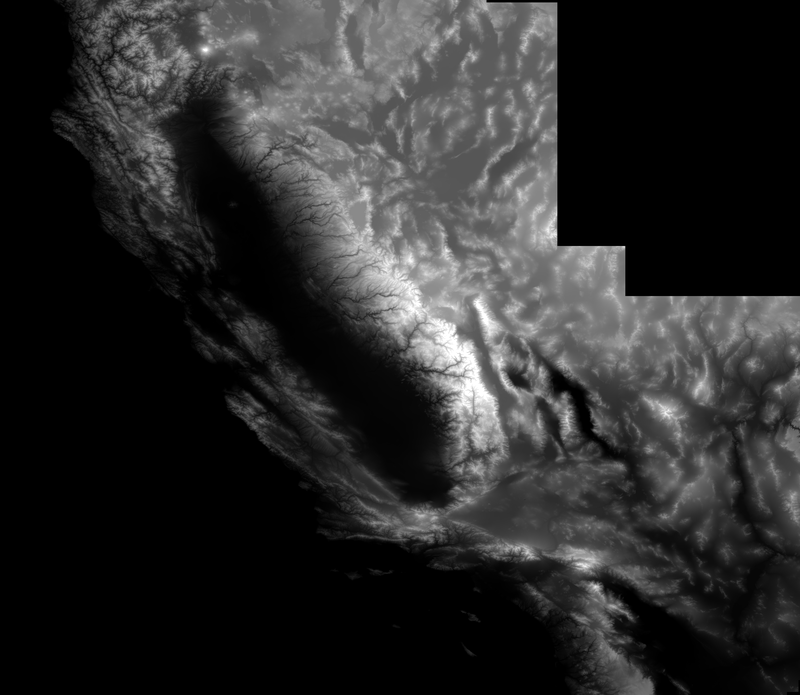
The other units in there are under the "Coordinate System is" section, and are meters, and relative to the World Geodetic System 1984 datum; this refers to height; the very last line is the lowest and highest points in file, in meters from that WGS84 baseline. If you were to view the file as though it were an image, it would look like this:

^{_{if you squint, you can kinda see the mountains}}

This is because the highest possible value an image like that could have for a pixel is 65,535, and the highest point in our dataset is only 4,412, which is not that much in comparison. Plus, it includes portions of not-California in the height data, and ideally, we want those places to be 0; we have a little more processing to do before we can use this.

Thank you, State of California!

The first order of business is to mask out everything that's not California, and the first thing I needed for that was a shapefile that described the California state border. Luckily, that exact thing is publicly available from the state's website!

Test prints

Give it a good smear

Final cut

Thank yous, lessons learned, and open questions

thank you: wife, steve at the shop, friends indulging my oversharing, NASA, Blender, FreeCAD

lesson: I started basically knowing nothing, but now retracing my steps I feel like I understand everything much better than when I was first racing through the domain trying to get to a point where I could just produce the artifact.

lesson: pipeline of geotiff -> mask -> scaled heightmap -> mesh -> solid body

lesson: see whole article about GIS stuff

question: could I do it better in blender? freecad? could I have used gdal_polygonize (doubtful, given how much I had to blur and decimate)?

I'm pretty sure this is more "represent shapes with math" than with a computer, but the computer is helping us do the math and it's more relatable. ↩︎
I think you could also have a 2D sheet with a hole cut out of it represented by a mesh that is manifold, as long as the connectivity was correct in terms of how many shared edges and vertices there were (though this would not be a valid STL file). Imagine a cloth sheet with a hole cut out in the middle, and the edge of the hole hemmed or otherwise "sealed", which is then a manifold boundary. See this powerpoint deck for a pretty math-y overview of "mesh basics" (but not really that basic, that's just academics trolling us, don't let it bother you). If I'm wrong about a 2D sheet with a hole being possibly manifold, I invite correction! ↩︎
A classic example of Chekhov's Scarce Computational Resource. ↩︎
Each pixel is 16 bits, so the possible values are from 0 to 2^16 - 1. 2^16 is 65536, so there you go. ↩︎
Technically, it's an arc along the WGS84 ellipsoid, which is a perfectly smooth smushed sphere, which more closely matches the real shape of the Earth vs. a perfect sphere. ↩︎

15 KiB Raw Blame History Unescape Escape